NOMAD Datasets and Calibration Steps

 

 

 

1. Introduction

NOMAD can make a wide variety of observations, for example: occultation, dayside nadir, limb, etc; and for each observation it can measure in one of many different measurement acquisition types. This document aims to:

• Explain how each observation/measurement type is made
• Give a list of possible advantages/disadvantages and limitations of each type
• Explain how the data pipeline processes the data
• Describe how the data is stored within the hdf5 files made available to the science team

1.1 Possible Observation Types

Observation Types	Description
Ingress solar occultation	Normal solar occultation starting when the line of sight is above the atmosphere and ending when sun is blocked by the surface.
Egress solar occultation	Normal solar occultation starting when the line of sight to the sun is blocked by the surface and ending when it is above the atmosphere.
Merged solar occultation	Double solar occultation, consisting of an ingress, starting above atmosphere, and an egress, ending above atmosphere. These occur when there is insufficient time between the ingress and egress to cool down the infrared detector for the second measurement, and are split into normal ingress and egress occultations.
Grazing solar occultation	Solar occultation where, due to orbital geometry, the sun is never blocked by the surface. Starting above the atmosphere, the line of sight passes through the atmosphere to a minimum altitude, then increases to end above the atmosphere.
Dayside Nadir	Nadir measurement on the illuminated side of the planet. Observations can be of variable length, beginning and ending near the nightside terminator to cover the whole dayside, or shorter and centred on the subsolar latitude. Can also be split into 3 separate measurements.
Nightside Nadir	Nadir measurement on the nightside of the planet.
Limb	Measurement of the illuminated limb of the planet.
Phobos	Measurement of the moon Phobos
Deimos	Measurement of the moon Deimos
Calibration	Many types e.g. sun pointing, solar line scan, etc.

 

1.2 Possible Measurement Types

Measurement Types - SO/LNO Channels	Description
Solar occultation (50km switch)	5 diffraction orders + 1 dark per second. When the line of sight reaches 50km , the combination of diffraction orders being measured is changed. No onboard background subtraction.
Solar occultation (0-250km)	5 diffraction orders + 1 dark per second, same order selection throughout. No onboard background subtraction.
Solar occultation (50km switch, dark subtraction)	6 diffraction orders per second, diffraction order selection changed at 50km. Dark frames subtracted onboard.
Solar occultation (0-250km, dark subtraction)	6 diffraction orders per second, same order selection throughout. Dark frames subtracted onboard.
Nadir	Nadir measurement of 2 to 6 diffraction orders per 15 seconds, dark subtracted onboard.
Limb	Limb measurement of 2 diffraction orders per 15 seconds, dark subtracted onboard.
ACS Boresight Limb	Special limb measurement of 2+ diffraction orders, measured during an ACS/MIR or ACS/TIRVIM solar occultation where line of sight is pointed close to the sun but not directly at the solar disk. Onboard dark subtraction.
Fullscan (slow)	Nadir, limb or occultation diffraction order stepping over any range/number of orders, dark subtracted onboard.
Fullscan (fast)	Solar occultation order stepping over any range/number of orders at a high cadence rate, dark subtracted onboard.
Calibration	Many types e.g. line of sight, solar fullscan, solar miniscan, integration time stepping, etc.
Measurement Types - UVIS Channel	Description
Solar occultation (binned)	Detector pixel values are vertically binned onboard. 3 full or partial spectra are recorded per second. No dark subtraction is made onboard.
Solar occultation (unbinned)	Each pixel value is stored individually. Full or partial spectra can be transmitted to Earth at a variety of cadence rates. No dark subtraction is made onboard.
Nadir (binned)	Detector pixel values are vertically binned onboard. Full or partial spectra can be transmitted to Earth at a variety of cadence rates. Occasional dark frames are taken and transmitted to Earth
Nadir (unbinned)	Each pixel value is stored individually. Full or partial spectra can be transmitted to Earth at a variety of cadence rates. Occasional dark frames are taken and transmitted to Earth.
Calibration	Many types e.g. line of sight, integration time tests, etc.

 

1.3 Nominal Observations

The table below shows the nominal observation types made by NOMAD. These make up the vast majority of all observations, and the calibration of these takes priority. Other observations will eventually be calibrated (where possible) in future updates.

Channel	Observation Mode	Measurement Type(s)	Description
SO	Ingress	Solar occultation, 0-250km, or 0-50km and 50-250km	5-6 diffraction orders
	Egress	Solar occultation, 0-250km, or 0-50km and 50-250km	5-6 diffraction orders
	Merged	Solar occultation, 250km-0-250km	5-6 diffraction orders. Occultations will be split into Ingress and Egress
LNO	Dayside Nadir	Nadir, observation centred on surface point with lowest solar incidence angle	1-6 diffraction orders
UVIS Occultation	Ingress	Solar occultation, 0-250km	Detector can be horizontally binned or unbinned
	Egress	Solar occultation, 0-250km	Detector can be horizontally binned or unbinned
	Merged	Solar occultation, 250km-0-250km	Detector can be horizontally binned or unbinned. Occultations will be split into Ingress and Egress
UVIS Nadir	Dayside Nadir	Nadir, observation centred on surface point with lowest solar incidence angle	Detector can be horizontally binned or unbinned

1.4 Observation Type Letters

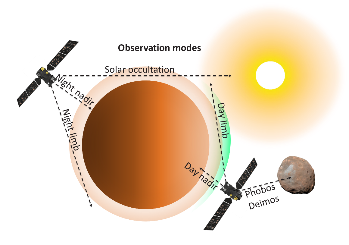
Figure 1: NOMAD observation modes

 

Every NOMAD HDF5 file is given a letter to denote the type of observation. The following observation types are defined for NOMAD. These can be split into science observations, where each type is assigned a letter, and calibration observations, which are assigned the letter C:

 

I = Ingress solar occultation.

NOMAD performs an observation during a sunset, where TGO points the boresights to the centre of the Sun. The observation will start some minutes before the line of sight enters the atmosphere (full sun reference spectra) and will continue some minutes after the line of sight has hit the Martian disk (dark spectra). These are standard science measurements where for SO a small selection of diffraction orders are cycled through repeatedly. This is the baseline science observation during an ingress.

E = Egress solar occultation.

NOMAD performs an observation during a sunrise, where TGO points the boresights to the centre of the Sun. The observation will start some minutes before the line of sight leaves the Martian disk (dark spectra) and will continue some minutes after the line of sight has left the atmosphere (full sun reference spectra). These are standard science measurements where for SO a small selection of diffraction orders are cycled through repeatedly. This is the baseline science observation during an egress.

G = Grazing solar occultation (currently only applies to SO data in levels 0.3K and above).

TGO points the boresights to the centre of the Sun, except in this case the line of sight never intersects the planet’s surface due to the Sun-Mars-satellite geometry. The observation begins above the atmosphere and ends above the atmosphere. Due to the lack of dark spectra, an error is not calculated and therefore these observations do not pass through the data pipeline. Data will be made available when a calibration routine is ready. At present these observations are not converted to transmittance by the pipeline, though the other calibrations are applied. Prior to level 0.3K, grazing and merged occultations are given the letter I.

S = Fullscan (SO/LNO only, during a solar occultation observation).

TGO points the NOMAD boresights to the centre of the Sun during this observation. This has to be done while the FOV passes through the atmosphere, i.e. a normal Ingress or Egress observation has to be sacrificed, or the fullscan has to be combined with the Ingress or Egress observation (only during a long occultation at high beta angle). The SO or LNO channel will perform a sweep over the complete or a subset of the spectral range, one diffraction order at a time. These measurements could be calibrated spectrally and radiometrically, but will not typically pass through the occultation pipeline. If operating simultaneously, UVIS will observe in normal Ingress or Egress mode during this time: a fullscan does not apply to UVIS.

F = Fullscan (SO/LNO only, during a nadir observation).

TGO will point the NOMAD nadir boresights to nadir during this observation, i.e. a normal dayside or nightside nadir observation has to be sacrificed. The LNO channel will perform a sweep over its complete or a subset of the spectral range, one diffraction order at a time. These measurements can be calibrated spectrally and radiometrically, but will not typically pass through the nadir pipeline (they are typically used for testing purposes). If operating simultaneously, UVIS will observe in normal nadir mode during this time: a fullscan does not apply to UVIS.

D = Dayside nadir.

TGO will be in its nominal pointing conditions, i.e. the –Y direction is aimed approximately towards the centre of Mars, perpendicular to the surface directly underneath it. The sun is positioned such that the surface is illuminated. In principle NOMAD can measure with LNO and UVIS at any time that the TGO axis is pointing nadir. These are standard science measurements where for LNO a small selection of diffraction orders are cycled through repeatedly. This is the baseline science observation during a nadir.

N = Nightside nadir.

TGO will be in its nominal nadir pointing condition, i.e. –Y direction approximately towards the centre of Mars. The region of the surface in nadir is in darkness. These are standard science measurements where for LNO a small selection of diffraction orders are cycled through repeatedly. This is the baseline science observation during a nadir.

P = Phobos

TGO will point a nadir boresight (typically either LNO, UVIS or the spacecraft -Y) towards the moon Phobos. LNO performs either a standard science measurement, usually with a reduce field of view, where a small selection of diffraction orders are cycled through repeatedly, or a fullscan over a subset of the spectral range, one diffraction order at a time. UVIS typically observes in full frame mode, as the moon is small and so the signal does not fill the entire field of view.

Q = Deimos

TGO will point a nadir boresight (typically either LNO, UVIS or the spacecraft -Y) towards the moon Deimos. LNO performs either a standard science measurement, usually with a reduce field of view, where a small selection of diffraction orders are cycled through repeatedly, or a fullscan over a subset of the spectral range, one diffraction order at a time. UVIS typically observes in full frame mode, as the moon is small and so the signal does not fill the entire field of view.

L = Limb

One or more NOMAD channel FOVs will be pointed towards the limb of Mars. This can be achieved by rotating the spacecraft, so that the nadir (-Y) face of the spacecraft is pointed to the limb, or for LNO by using the occultation channel whilst not pointed to the sun. These are standard science measurements where a small selection of diffraction orders are cycled through repeatedly, and measurements will be calibrated using the nadir pipeline.

C = Calibration

This type encompasses all calibration measurements, which are given a secondary letter to distinguish the calibration type:

• CL = Pointing calibrations, where TGO performs a line or raster scan around a target (typically the Sun). From these measurements the misalignment can be calculated between the S/C pointing axis and the NOMAD boresights. This misalignment value will be used afterwards to correct the S/C pointing vector.

• CF = Fullscans (SO/LNO only), but when the FOV does not pass through the atmosphere. The S/C will point a boresight to the centre of the Sun during this observation, which can be done at any time when the Sun is visible. The NOMAD SO and/or LNO channels will perform a sweep over their complete spectral range. These measurements can be calibrated spectrally but not radiometrically.

• CM = Miniscans (SO/LNO only), where the channels will perform a sweep over a fraction of their spectral range whilst pointing towards the sun (but when the FOV does not pass through the atmosphere). These are used for spectral calibration, namely to generate a set of coefficients to calibrate all the other observations. These measurements can be calibrated spectrally but not radiometrically.
• CS = Solar/dark sky stare. The channel observes the Sun for an extended period of time; this is occasionally performed by UVIS during an SO/LNO solar fullscan or miniscan observation. The SO and LNO channels can performed an integration time stepping observation, where the integration time is gradually increased so that the saturation time can be determined. Channels may be pointed towards the Sun or dark sky. These measurements can be calibrated spectrally but not radiometrically.

 

 

 

1.5                    Data Pipeline Overview

 

The data pipeline is split into major and minor levels. Major levels are denoted by a number, and minor levels by a letter. In general, the philosophy is that each manipulation of a dataset should be easily traceable between levels, and so the values in a dataset should not be changed multiple times within a single level.

The products of the major levels are as follows:

• Level 0.1: HDF5 file structure made and basic detector corrections applied
• Level 0.2: Geometry added. UVIS detector corrections.
• Level 0.3: Spectral and more advanced calibrations applied
• Level 1.0: Radiometrically calibrated data

Within the major levels, the minor levels are given letters. Note that, as levels are merged and moved, some letters are omitted (however the levels are always in alphabetical order). The UVIS pipeline deviates slightly from this, as the geometry is added before detector corrections in level 0.2.

 

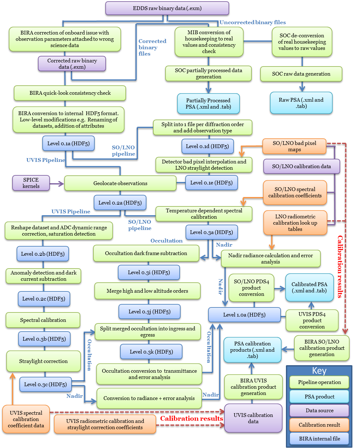
Figure 2: Data pipeline outline

 

 

2 Data Pipeline Processing of Observations

Every HDF5 file has an observation type letter in its name. As can be seen above, there are many many possible combinations of observation and measurement types; far too many to assign a letter to each. The observation type letter can be used to find certain observation types, but the primary use is to direct the file through the correct branch of the data processing pipeline.

2.1 Level 0.1A

2.1.1 Housekeeping calibration

Conversion of housekeeping to physical units

2.2                Level 0.1D

2.2.1         Split by diffraction order

All SO/LNO files, except fullscans, are split into one file per diffraction order. If the diffraction orders are switched at 50km, then two sets of files are created and appended by _1 or _2, where 1 is chronologically first (i.e. high altitudes for an ingress, low altitudes for an egress). If no switch is made, _1 is appended.

2.2.2        Expand filenames

Observation type letter and diffraction order added to filename. Naming now follows the following convention:

• YYYYMMDD_hhmmss_Level_Channel_OrderSet_ObservationTypeLetter_DiffractionOrder.h5
• YYYYis the observation start year
• MMis the observation start month
• DDis the observation start date
• hhis the observation start time hour
• mmis the observation start time minute
• ssis the observation start time second
• Levelis the data level with a letter p to replace the point, e.g. 0p1a, 0p3a, 1p0a, etc.
• Channelis either SO, LNO or UVIS
• (SO/LNO only)OrderSet is either 1 or 2 indicating the set of diffraction orders used. The orders can change during an occultation, therefore the first set is 1 and the second set is 2. If the same order combination is used throughout, this is always 1.
• ObservationTypeLetter (see 1.4, note that G does not apply here)
• (SO/LNO only and not for fullscans)DiffractionOrder is the diffraction order

Note that the above convention is slightly modified for SO files at the end of Level 0.3k, due to the splitting of merged occultations and OrderSet transition.

 

Level 0.1E - LNO straylight

Straylight can be observed in the data when the LNO channel is observing in nadir and the spacecraft is in a particular geometry which only occurs when slewing to an ACS solar occultation. This happens only on the nightside of the planet and so no science is lost. However, a signal is observed in the data, and so the affected frames are removed to avoid misinterpretation of the spectra.

 

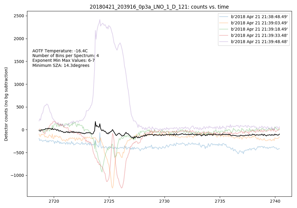
Figure 3: Solar straylight entering LNO has a huge impact on the signal. As LNO is background-subtracted, the straylight manifests itself as positive or negative values depending on whether it hits the detector during the dark or measurement frame.

Frames containing this straylight are removed automatically, based on a set of detection criteria - i.e. spacecraft orientation with respect to the Sun, and anomalous detector values. The frames directly before and after are also removed, to ensure that all incorrect data is removed.

The data is not recoverable when straylight is present, and so all radiance values in the affected frames are set to NaN. The field YValidFlag is used to indicate which spectra are valid, where:

1 = spectrum is valid

0 = spectrum is invalid

Assuming straylight has been detected in measurement frame 4, the data would be as shown in Table 1.

 

LNO Radiance
Measurement 1, Pixel 1 Value	Pixel 2 Value	...	Pixel 320 Value
Measurement 2, Pixel 1 Value	Pixel 2 Value	...	Pixel 320 Value
NaN	NaN	...	NaN
NaN	NaN	...	NaN
NaN	NaN	...	NaN
Measurement 6, Pixel 1 Value	Pixel 2 Value	...	Pixel 320 Value

YValidFlag

1

1

0

0

0

1

Table 1: Radiance and YValidFlag fields, showing how the data is modified if straylight is detected in measurement 4.

 

 2.2.3        SO non-linearity

The SO non-linearity correction has been de-activated after it was causing issues with the data.

The SO and LNO detectors and readout electronics have a slightly non-linear response the radiance when the incident radiance is very small. The SO channel observes the sun during a solar occultation, and so low integration times (~4ms) are used to avoid saturation. This means that when the input radiance is low (e.g. when viewing the lower atmosphere, or planet, or when taking a dark frame) then the signal could be within the non-linear region. This never applies to LNO nadir or limb data, as the lower signal means that the long integration times (~200ms) are required. The correction is derived from integration time stepping measurements viewing dark space.

 Figure 4: Integration time vs counts for one SO channel pixel, acquired when observing dark space. The dots indicate the linear line of best fit. The non-linear region is magnified for clarity.

The integration time is stepped from 0 to 1400ms, and a linear fit is made to the data from 200-1400ms to calculate the difference between expected and measured counts in the non-linear region. This is done for every pixel individually, though the variation between pixels is very small. Figure 2 shows the deviation from non-linearity for a single pixel - the region is compared to the entire detector region (a pixel saturates around 12000 counts), and when zoomed in the deviation from the linear fit remains small.

Every detector count is checked to see if the value is within the non-linear region. If so, that value is replaced by the linear-equivalent value from the line of best fit.

 2.2.4        Level 0.1E - SO/LNO bad pixel

 

Figure 5: SO bad pixel map. White dots indicate bad pixels. Two observations were required to cover all the pixels required, hence the small difference between the top and bottom rows is likely due to slightly different instrument temperature.

 

Bad pixels were determined by analysing a subset of spectra and finding the pixels that behave anomalously compared to adjacent pixels throughout a measurement. This method works even for the narrowest absorption lines, as there is always a spectral overlap between consecutive pixels, and so an anomalous value in one pixel only can only be due to the pixel, not the atmosphere or surface of Mars.

If a pixel behaves anomalously the value is corrected by linearly interpolating from adjacent pixels. Pixels at the edge of the detector, where the signal is already very small, are given the same value as the adjacent pixel. It should be noted that some bad pixels only give anomalous readings occasionally, and so some spectra can still contain spikes after transmittance/radiance calibration.

 2.2.5         Level 0.1E - LNO detector offsets

 

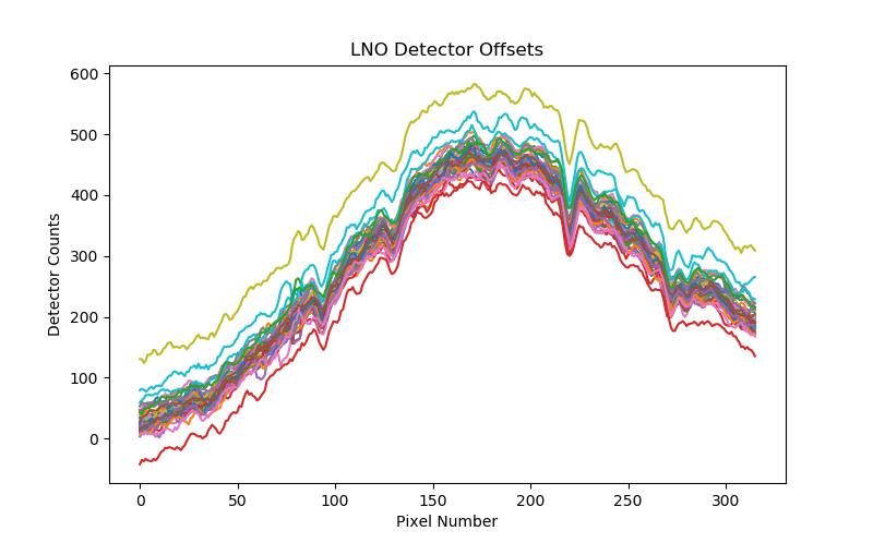
Figure 6: LNO detector spectra before offset correction

The zero offset level can shift up and down due to the detector grounding and the very small values generated by a nadir measurement (Figure 4). To correct this, an offset correction is calculated from the mean of the first 50 pixels. The offsets are subtracted from each spectrum to remove the anomalous offset, as shown in Figure 5.

 

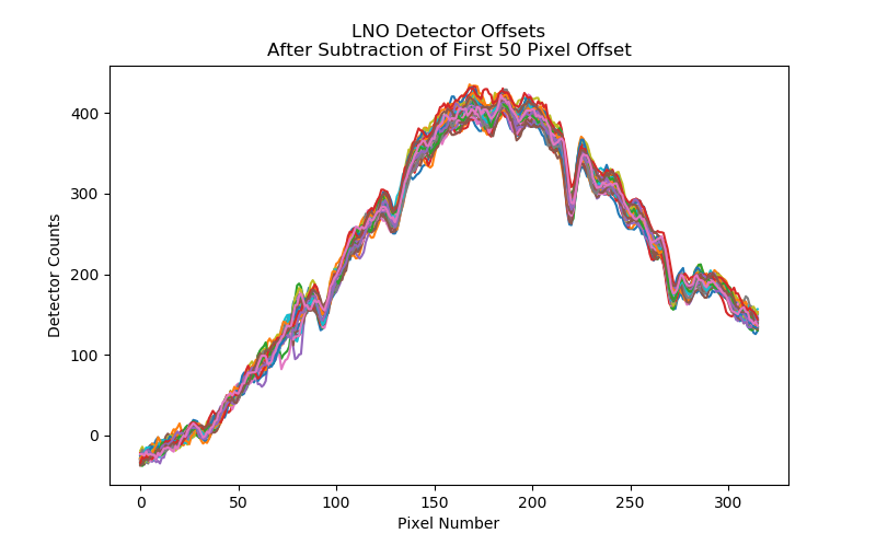
Figure 7: LNO nadir spectra after subtraction of the offset. A second offset is added to shift the curve upwards, removing the negative counts in the first pixels.

 

Removing the offset means that the first pixels can be less than zero, therefore a second offset is subsequently added to the data. This offset is derived from solar calibration measurements of the same diffraction order, where a ratio is calculated between the mean of the centre pixels [160-240] and the mean of the first 50 pixels when pointing at the sun. An offset is then added to each nadir spectrum so that the same ratio is present in the data.

 

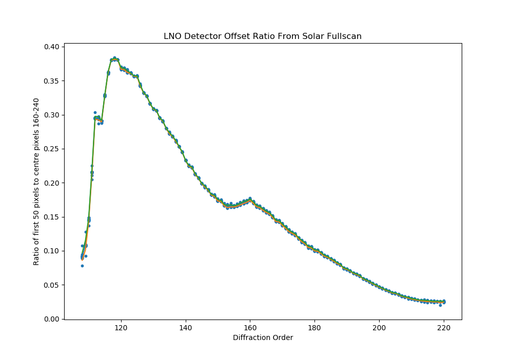
Figure 8: Ratio of mean value of first 50 pixels to mean value of pixels in centre of detector, calculated from viewing the sun for each diffraction order. This ratio is then applied to the data, shifting the nadir curves upwards so that the same ratio is observed in the spectra.

 

2.2.6        Level 0.1E - LNO nadir data vertically binned

The SNR of the LNO channel is low when observing in nadir, and so the spectra measured for each detector bin (of the same measurement) must be summed together to produce one spectrum.

 

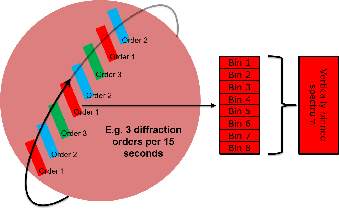
Figure 9: Vertical binning of one LNO nadir detector frame (red). Here 3 diffraction orders are measured, generating 8 individual spectra for a given measurement.

The SO and LNO channel always return 24 lines per measurement period (where the period is 1 second for occultation or 15 seconds for nadir observations). Therefore here, 3 orders are measured per period and so 8 spectra are returned per order. If 4 orders were measured, 6 spectra would be returned; if 2 orders then 12 spectra would be returned, etc. The 6, 8 or 12 LNO nadir spectra are then vertically binned to give a single spectrum per order per measurement period (Figure 7).

The detector bins observe different locations on the planet, but this spatial information is lost when the data is binned - though individual bins do not have sufficient signal to be scientifically useful.

2.2.7         Level 0.1E - SO/LNO detector bins flattened

SO and LNO radiance/transmittance values are converted from a 3D array (size = number of observations x number of bins x 320 pixels) to a 2D array (size = [number of observations x number of bins] x 320 pixels). BinStart and BinEnd fields contains the start and end detector row for each bin. LNO nadir observations have already been vertically binned into a 2D array, and so the radiance values remain unchanged.

 

 

2.2.8        Level 0.2A – Geometry overview

There are three types of shape models used to calculate geometric parameters:

• Ellipsoid- this is the most basic shape model, where Mars is modelled as a tri-axial ellipsoid of radii 3396.19km x 3396.19km x 3376.2km
• Areoid- this is the equivalent to a "sea level" for Mars, where the gravitational and rotational potential is constant across the entire surface. The zero level is defined by MGS/MOLA using a 4 pixels per degree model
• Surface- this is the real surface elevation, calculated from a digital shape kernel (DSK) by MGS/MOLA at a resolution of 4 pixels per degree using the MGM1025 model (Lemoine et al., 2001).

 

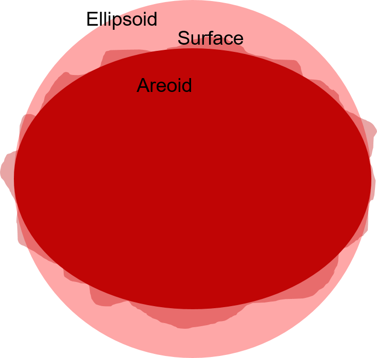
Figure 10: Pictorial representation of the difference between ellipsoid, surface and areoid geometries.

 

 

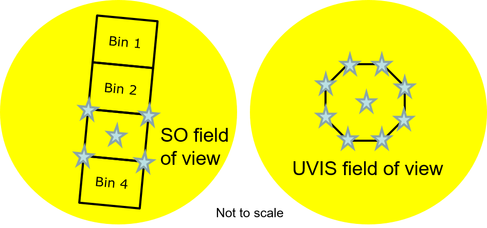
Figure 11: SO and UVIS solar occultation geometry, showing the 5 points per bin for SO and 9 points for UVIS.

 

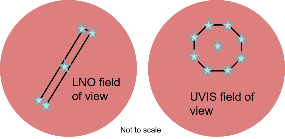
Figure 12: LNO and UVIS nadir geometry, showing the 5 points per bin for SO and 9 points for UVIS

 

Geometry is stored for each pointing direction (Figure 9 and Figure 10). There are 5 points for SO/LNO solar occultations and nadir observations:

• Point0is the centre of the entire field of view of the bin
• Point1to Point4 define the corners of the field of view of the bin.

UVIS has a circular aperture, defined by 9 points:

• Point0is the centre of the field of view
• Point1to Point8 form an octagon around the field of view edge.

As described above, the LNO nadir frame has been vertically binned, and so there is effectively just one bin per measurement. Therefore points 1-4 define the corners of the entire LNO field of view.

The fields of view of the bins are defined using points as shown in Figure 11. Relevant geometric parameters, such as latitude, longitude and viewing angle information are calculated for each point. The relative x and y positions of each point (the numbers in brackets in Figure 11) are given in the fields PointX0, PointY0, PointX1, PointY1, etc. Their direction is defined by the SPICE instrument kernel reference frame for each channel, where X points along the long edge of the SO/LNO slit and Y the short edge.

UVIS field of view

SO/LNO field of view

Point2 (-1/√2, +1/√2)

Point3 (0, -1)

Point3 (0, -1)

Point2 (-1/√2, -1/√2)

Point2 (+1/√2, -1/√2)

Point3 (+1, 0)

Point2 (+1/√2, +1/√2)

Point1 (0, +1)

Point0 (0, 0)

Point0 (0, 0)

Point1 (+1, +1)

Point4 (+1, -1)

Point2 (-1, +1)

Point3 (-1, -1)

 

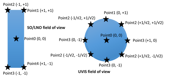
Figure 13: Geometry points as defined in relation to the channels' fields of view.

 

Some geometric parameters do not depend on pointing direction, for example SubObsLat and SubObsLon. Start and end values are recorded per spectrum acquired, i.e. SubsObsLatStart and SubObsLatEnd.

Some geometric parameters have different values depending on the point – therefore there are two values (start and end times) per point per spectrum acquired. An integer is appended to the field name to indicate the point number, e.g. LonStart3 and LonEnd3 are the start and end longitudes for point 3.

Using the surface shape model means that the geometric surface parameters EmissionAngle (angle between surface normal and spacecraft), PhaseAngle (angle between sun, surface and spacecraft) and SunSZA (angle between Sun and surface normal) are based on the real surface contours rather than a reference ellipsoid. SurfaceRadius is the height of the shape model surface above the centre of the planet, so that users can reference the surface height to the absolute position of Mars. The SurfaceAltAreoid field is the height of the surface above the reference areoid, which defines the relative atmospheric pressure at the surface. All of the fields above are point-dependent, e.g. EmissionAngle is defined as EmissionAngle0Start, EmissionAngle0End, EmissionAngle1Start, etc. In nadir, latitude and longitude are effectively independent of shape model and hence are provided for ellipsoid model only.

In solar occultation mode, the geometry is defined at the tangent point, i.e. the point on the Mars ellipsoid closest to the line of sight vector of each point. Each shape model has a different tangent height, and so TangentAlt (height above reference ellipsoid), TangentAltAreoid (height above areoid) and TangentAltSurface (height above surface shape model) are all defined separately. SurfaceRadius and SurfaceAltAreoid are also given so users can convert between the three types. All are given separately for the start and end time of each field of view point.

LST is the local solar time, in hours, defined using the SPICE kernel definition = 12 + (surface longitude for a point – solar longitude)/15

LSubS, the planetocentric solar longitude, commonly referred to as Ls (pronounced "L sub S", or "L-S"), is the position of Mars relative to the Sun measured in degrees from the vernal equinox (start of northern Spring). This number is used as a measure of Martian seasons: Northern Spring/Southern Autumn start at 0°, Northern Summer/Southern Winter start at 90°, Northern Autumn/Southern Spring start at 180°, and Northern Winter/Southern Summer begin at 270°.

Information on the spacecraft position and relative speed is also provided, such as DistToSun (distance from spacecraft to sun in AU), SpdObsSun (relative velocity of spacecraft from Sun), SpdTargetSun (relative velocity of Mars from Sun), ObsAlt (altitude of spacecraft above Mars centre), also position of spacecraft and sun above Mars in fields SubObsLon, SubObsLat and SubSolLon, SubSolLat. These parameters are independent of spacecraft pointing, and therefore have two values (start and end of each measurement) per measurement.

Invalid values are set to -999.0. This could occur, for example, when the solar occultation boresight is pointing towards the surface (therefore tangent altitude is invalid) or if the nadir channel points off-planet during an observation, which can happen if the spacecraft is slewing to/from another measurement.

2.2.8.1   SO/LNO Occultation (50km switch)

 

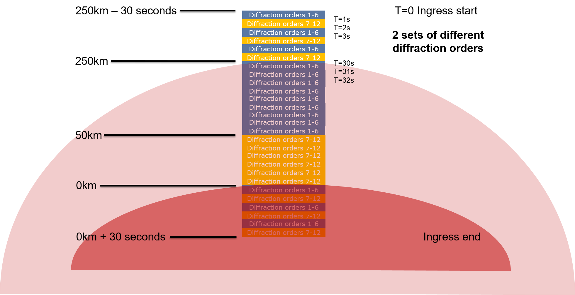
Figure 14: Diagram showing the SO data acquired during a solar occultation where the set of diffraction orders is changed 50km above the surface.

 

2.2.8.2  SO/LNO Occultation (0-250km)

 

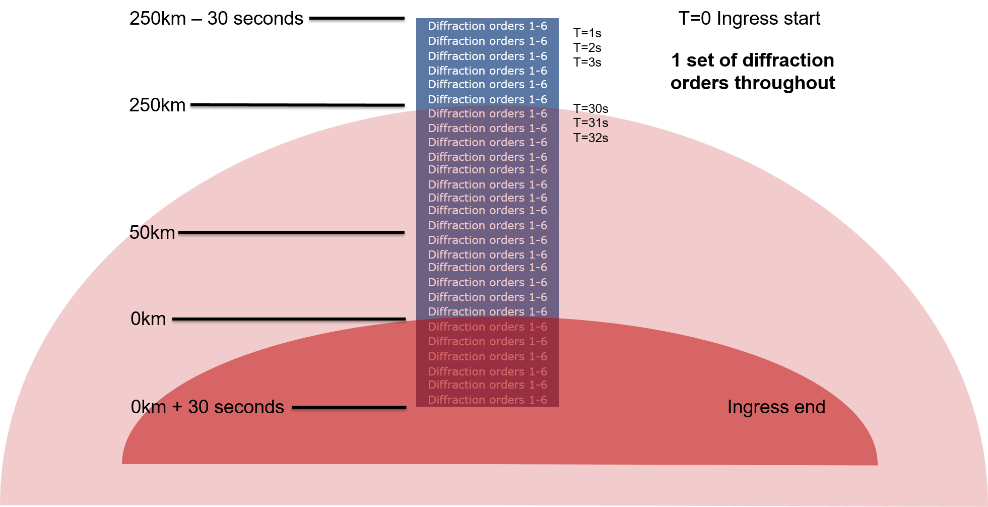
Figure 15: An SO occultation where the same diffraction orders are measured throughout.

 

Figure 14 and Figure 15 show the principal two types of solar occultations measured by the SO channel. Note that, in cases where onboard dark subtraction is switched off, diffraction orders 6 and 12 are normally dark frames, hence only 5 or 10 diffraction orders are measured.

The SO data has been flattened into a 2D array (section 2.2.7), and so the data is now in the format shown in Table 2, with one spectrum per bin per measurement per row. For each transmittance spectrum there is a BinStart and BinEnd value to specify the detector rows used to acquire that bin.

SO Transmittance
Measurement 1, Bin 1, Pixel 1	Pixel 2	...	Pixel 320
Measurement 1, Bin 2, Pixel 1	Pixel 2	...	Pixel 320
Measurement 1, Bin 3, Pixel 1	Pixel 2	...	Pixel 320
Measurement 1, Bin 4, Pixel 1	Pixel 2	...	Pixel 320
Measurement 2, Bin 1, Pixel 1	Pixel 2	...	Pixel 320
Measurement 2, Bin 2, Pixel 1	Pixel 2	...	Pixel 320

BinStart	BinEnd
Bin 1 Detector Row Start	Bin 1 Detector Row End
Bin 2 Detector Row Start	Bin 2 Detector Row End
Bin 3 Detector Row Start	Bin 3 Detector Row End
Bin 4 Detector Row Start	Bin 4 Detector Row End
Bin 1 Detector Row Start	Bin 1 Detector Row End
Bin 2 Detector Row Start	Bin 2 Detector Row End

Table 2: SO transmittance and binning data.

 

2.2.8.3  LNO nadir

Due to the low SNR in nadir mode, all the LNO bins have been summed into a single spectrum per measurement. Therefore, in the absence of separate bins, the tabulated data contains just one spectrum per measurement. BinStart and BinEnd therefore are the same for all measurements and reflect the start and end row of the detector readout.

 

LNO Radiance
Measurement 1, Pixel 1	Pixel 2	...	Pixel 320
Measurement 2, Pixel 1	Pixel 2	...	Pixel 320
Measurement 3, Pixel 1	Pixel 2	...	Pixel 320
Measurement 4, Pixel 1	Pixel 2	...	Pixel 320

BinStart	BinEnd
Detector Row Start	Detector Row End
Detector Row Start	Detector Row End
Detector Row Start	Detector Row End
Detector Row Start	Detector Row End

Table 3: LNO radiance and corresponding binning data

 

2.2.8.4  UVIS Nadir and Occultation

UVIS acquires one spectrum per measurement, with no bins or diffraction orders.

 

UVIS Transmittance/Radiance
Measurement 1, Pixel 1	Pixel 2	...	Pixel 1048
Measurement 2, Pixel 1	Pixel 2	...	Pixel 1048
Measurement 3, Pixel 1	Pixel 2	...	Pixel 1048
Measurement 4, Pixel 1	Pixel 2	...	Pixel 1048
Measurement 5, Pixel 1	Pixel 2	...	Pixel 1048

Table 4: UVIS transmittance data for a full spectrum (1048 pixels)

 

2.2.8.5  LNO Limb

At the time of writing, only the LNO channel can observe the limb using its flip mirror while the spacecraft continues in nadir pointing mode. The signal entering the UVIS solar occultation boresight is attenuated, and so the spacecraft must be orientated with the nadir channel pointing towards the limb for both LNO and UVIS to measure it.

LNO observes the limb passively, with no control over pointing, and so the pointing can vary between and within observations. In future it is hoped that the limb can be measured in a controlled way, viewing at a fixed altitude, or with the UVIS nadir boresight.

 

Figure 16: An LNO limb observation using two diffraction orders. The FOV generally sweeps across the limb as the spacecraft moves, in the direction of the short edge of the slit.

 

The LNO limb data is arranged like SO/LNO solar occultations, split into bins and using the same geometric parameters, even though the SNR is too low per bin to be usable for science. This is because the altitude information is lost if the entire detector is binned, and so the SNR should be increased by summing each bin in time for a given altitude range.

 

 

Level 0.3A - SO/LNO spectral calibration

 

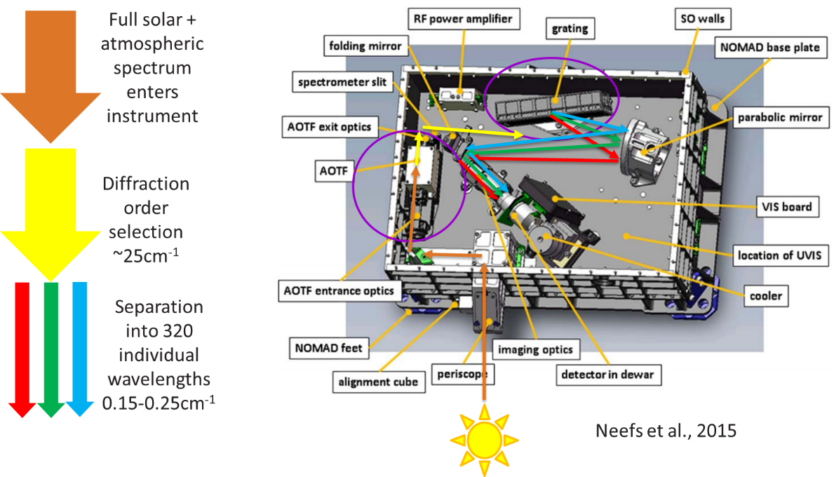
Figure 17: SO/LNO optical layout. A broad spectrum of infrared radiation enters the instrument; the AOTF selects a limited spectral range corresponding to a diffraction order; and the grating splits the radiation within the diffraction order onto the 320 detector pixels

 

  

Spectral calibration of the SO and LNO channels is complicated by the presence of the AOTF and diffraction grating. Without an AOTF, there would be >100 diffraction orders hitting the detector simultaneously, and so attributing an absorption line to a specific wavelength would be impossible.

The AOTF solves this by permitting only a limited spectral range to pass through it. In an ideal situation, the AOTF transmittance would be a boxcar function, of width exactly equal to the spectral range of the desired diffraction order. However, in reality the AOTF has a more complicated shape, akin to a sinc² function, with sidelobes that allow radiance to pass through it and hit the detector from adjacent diffraction orders. Accurate calibration is essential, so that all features present in a spectrum can be attributed to the principal or adjacent diffraction orders – and the shape of the AOTF function is correct so that the absorption depths of those features can be correctly used to determine the concentration of gas species in the atmosphere of Mars. Similarly, accurate wavenumber calibration of the diffraction grating is required so that the features observed match those in spectroscopic databases. This is further complicated by the effects of instrument temperature – NOMAD is not kept at a fixed temperature, and the metal diffraction grating is mounted to the instrument structure, and therefore can expand and contract as the temperature changes. This results in a temperature-dependent wavelength shift which must be corrected by the spectral calibration calculation. AOTF shape coefficients and spectral resolution vary by diffraction order.

The spectral calibration is, and will be, continually refined during the mission, and so the calibration coefficients and equations are likely the change often. The current published coefficients can be found in Liuzzi et al. 2018, which were derived from solar calibration measurements taken from Mars orbit in 2016. The calibration takes a variety of forms, as detailed below. All coefficients are provided in the files.

 

AOTF Calibration

The AOTF function is centred on the desired diffraction order by driving it with a specific radio frequency. Note that the diffraction order m is always an integer, and the AOTF frequency is always chosen so that the peak AOTF function matches the centre of a diffraction order.

 

The relation between the AOTF centre (in cm^-1) and the wavenumber is given as:

AOTF(v) = G₀ + G₁A + G₂A²

 

Where AOTF(v) is the central wavenumber in cm^-1 and A the AOTF frequency in kHz. The coefficients are:

 

Coefficient	AOTF tuning relation
G0	305.0604
G1	0.1497089
G2	1.34082 x 10-7

 

The AOTF centre shifts with temperature according the following relationship:

AOTF(v) = AOTF(v) + ([coefficient] * [channel temperature] * AOTF(v))

 

Where the coefficient here is the AOTF frequency shift due to temperature [relative cm-1 from Celsius]  = -6.5278E-05 

 

The channel temperature is taken from Channel/MeasurementTemperature for solar occultations, and Channel/InterpolatedTemperature[i] for solar calibrations (where i is the spectrum index)

 

Following Villanueva et al. 2022, the AOTF shape is now a combination of a sinc² added to a wide Gaussian. The following coefficients are used:

 

Coefficient	0	1	2
Sinc width [cm-1 from AOTF frequency cm-1]	2.01730360E+01	7.47648684E-04	-1.66406991E-07
Sidelobe factor [scaler from AOTF frequency cm-1]	4.08845247E+00	-3.30238496E-03	8.10749274E-07
Asymmetry factor [scaler from AOTF frequency cm-1]	-1.24925395E+00	1.29003715E-03	-1.54536176E-07
Gaussian peak intensity [coefficients for AOTF frequency cm-1]	1.60097815E+00	-9.63798656E-04	1.49266526E-07

 

The following are calculated from the AOTF centre frequency in wavenumbers e.g.

Sinc width(v) = 2.01730360E+01 + 7.47648684E-04 * AOTF(v) - 1.66406991E-07 * AOTF(v)²

 

The width of the Gaussian is assumed to be 50cm^-1 centred at the peak of the AOTF

 

The AOTF is then defined from the four shape values as follows:

def sinc(dx,width,lobe,asym,gauss_peak):

            sinc = (width*np.sin(np.pi*dx/width)/(np.pi*dx))**2.0

            ind = (abs(dx)>width).nonzero()[0]

            if len(ind)>0: sinc[ind] = sinc[ind]*lobe

            ind = (dx<=-width).nonzero()[0]

            if len(ind)>0: sinc[ind] = sinc[ind]*asym

            sigma = 50.0

            sinc += gauss_peak*np.exp(-0.5*(dx/sigma)**2.0)

            return sinc

Where dx is the relative wavenumber from the AOTF peak

 

1.1.1.2      Grating Spectral Calibration

The wavenumber-pixel calibration is:

v_p = m (F₀ + F₁p + F₂p²)

 

Where v_p is the wavenumber in cm^-1 of detector pixel p in diffraction order m and F₀, F₁ and F₂ the coefficients of a second order polynomial derived from ground and in-flight spectral calibration campaigns. The coefficients are:

 

SO Coefficient	Pixel spectral calibration coefficient
F0	22.4701
F1	5.480E-04
F2	3.32E-08

 

The wavelength shift due to temperature is accounted for by modifying the values of p used in the equation above. The field FirstPixel specifies the first value, and so the values of p are [FirstPixel, FirstPixel + 1, FirstPixel + 2… to FirstPixel +319)

The value of FirstPixel is determined from the temperature of NOMAD at the start an observation, and varies linearly with instrument temperature T:

FirstPixel = Q₀ + Q₁T

 

Where T is the MeasurementTemperature and the coefficients are:

 

SO Coefficient	Temperature shift coefficient (px/°C)
Q0	0.0
Q1	-0.8276

 

At present, FirstPixel is constant throughout an entire observation, however in future this may be subject to change.

 

1.1.1.3      Grating Blaze Function Calibration

The SO and LNO gratings are more efficient in diffraction radiation towards the centre of a diffraction order rather than at the edges, according to the blaze function. This is modelled as a sinc² function:

Blaze = (w_p * (sin(pi * x / w_p) / (pi * x))²

 

where w_p is the width of the blaze function (also known as the free spectral range, FSR) and x is the relative wavenumber for each pixel from the blaze peak b_p.

 

The initial FSR or blaze width, w_p1(v) is defined as:

w_p1 (v) = W₀ + W₁ (AOTF(v) – 3700) + W₂ (AOTF(v) – 3700)² + W₃ (AOTF(v) – 3700)³⁺

 

Where the coefficients are:

 

SO Coefficient	FSR / blaze width coefficient (cm-1)
W0	2.25863468e+01
W1	9.79270239e-06
W2	-7.20616355e-09
W3	-1.00162255e-11

 

And the temperature-corrected FSR or blaze width, w_p(v)  is calculated as follows:

w_p(v) = w_p1(v) + w_p1(v) * [Y₀ + Y₁T + Y₂T²]

 

Where T is the MeasurementTemperature and the coefficients are:

 

SO Coefficient	FSR / blaze width relative frequency shift coefficients [shift/frequency from Celsius]
Y0	-1.90001923e-04
Y1	-2.30708836e-05
Y2	-2.44383699e-07

 

The blaze peak b_p is then simply the diffraction order * width of the FSR i.e. m * w_p(v)

 

1.1.1.4     Pixel ILS Calibration

The spectral resolution of a pixel in the SO channel is modelled as a combination of two Gaussians. This will be updated soon.

 

 

2.2.10   Level 0.2B - UVIS reshape dataset

If dataset is unbinned, remove unmeasured detector rows from old Y, YMask and YError datasets (size = number of observations x 256 x 1048) to reflect the detector region used (size = number of observations x [VSTART - VEND + 1] x 1048).
If detector is vertically binned, replace old Y (size = number of observations x 256 x 1048), YMask and YError by a single line per observation (size = number of observations x 1048).

 

 

2.2.11     Level 0.2B - UVIS dynamic range correction

When the detector is vertically binned, reconstruct the spectra correcting the jump bug. Due to a communication problem between the on board UVIS electronic and SINBAD, during the binning process, the signal is artificially reset to zero each time it reaches a threshold value of 2²⁰ counts (~10E5), causing jumps (up or down) in the spectra.

In a spectrum, large signal variations can only be due to an artificial jump or to the steep variations of the solar radiation, but not to the characteristics of the Martian atmosphere/surface that show smooth wavelength dependencies.

The routine perform a first loop by comparing the signal variation between a wavelength pixel and the next one. Two cases: 1) if solar radiation is known to be smooth between these wavelengths, a large signal variation (7E5) in the recorded spectrum is due to an artificial jump and is corrected. 2) If solar radiation is known to have a steep variation between these wavelengths, then we expect to have also a similar steep variation in the recorded spectrum. However, a steep increase (/decrease) is likely to produce a jump down (/up) as the chance of reaching the threshold greatly increases. Therefore, a signal decrease (/increase) where the solar radiation is supposed to increase (/decrease) is due to an artificial jump and is corrected.

Practically the first loop starts at the first wavelength pixel (i.e. in the UV around 200 nm where the signal is low and where no jump are supposed to occur), and goes iteratively towards the last wavelength (around 650 nm). The absence of jump in the very first wavelength is yet performed using the same method as the second loop, explained hereafter.

 

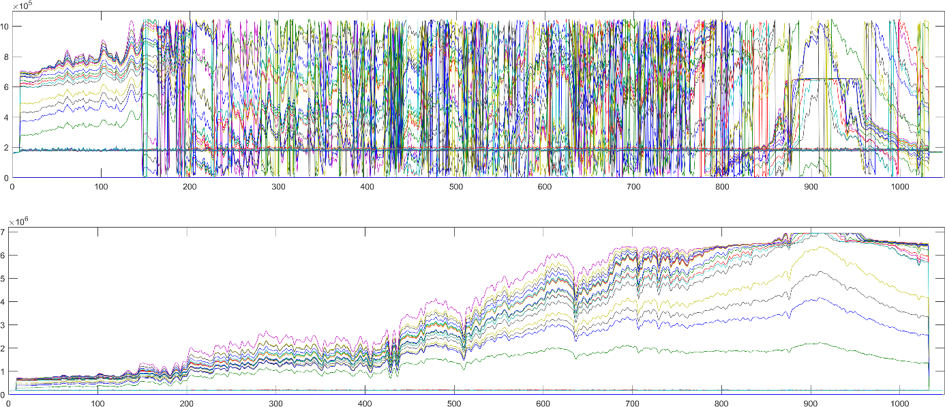
Figure 18: Raw spectra before (top) and after (bottom) dynamic range correction.

 

After the first loop, almost all jumps have been corrected. However, some particular jumps may subsist: these missed artificial jumps occur when the real variation is relatively large but not large enough so that the artificial jump is not exceeding the detection threshold.
A second loop is then performed and uses a comparison between the different spectra: it is performed knowing that the relative variations between two observations are supposed to be similar. Considering again one pair of adjacent wavelengths at a time, an important difference of the relative variation of two consecutive spectra indicate a missing jump.

 

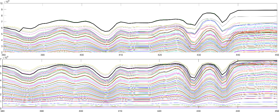
Figure 19: Example of jump corrected after the second loop of the dynamic range correction routine. Top: spectra after first loop. Bottom: spectra corrected after second loop.

 

 

2.2.12    Level 0.2B - UVIS detector saturation detection

Check for saturated pixels.
If detected, set relevant pixel in YMask to 2.
If detector is vertically binned, pixel saturation is detected only when all measured pixels of a column are saturated.

 

 

2.2.13    Level 0.2C - UVIS anomaly detection in dark measurements

Check the presence of anomalies at the pixel level in the dark measurement: detection of cosmic rays and hot pixels; update of the YMask (mask set to 3 for cosmic ray); a temporary dark measurement dataset, corrected for cosmic rays, is created and used in the next step of the dark current (DC) removal.

The routine uses comparisons between consecutive dark observations: dark measurements are supposed to be relatively constant over all pixels of a full CCD frame. Exceptions occur: 1) with “hot pixels” which behave differently than other pixels and 2) with cosmic ray hits on the CCD. The routine identifies these perturbed pixels and assigns them: as “hot pixels” when the pixel appear perturbed in several dark measurements and as “cosmic ray” when the pixel is perturbed in only one dark measurement.

The temporary dark measurement dataset created to be used in DC removal is obtained by replacing the values of all cosmic ray pixels by the mean on all non-perturbed pixels from the CCD frame of the dark measurement considered.

 

 

2.2.14    Level 0.2C - UVIS dark current removal

Removal of the dark current using the dark measurements (corrected for cosmic rays, cf. previous step) taken before and after a set of science frames. Knowing the temperature at which each science frame has been recorded, one linearly extrapolates a dark frame corresponding to this temperature between the two measured dark frames and subtracted it from the science frame.

Dark frame is set to zero in the Y dataset, bias and reverse clock are preserved.

 

 

2.2.15    Level 0.2C - UVIS anomaly detection

Check the presence of anomalies at the pixel level in the science measurements: detection of cosmic rays, dummy pixels and update of the YMask (mask set to 3 for cosmic ray). The routine uses comparisons between consecutive observations: it takes the ratio at all wavelengths between consecutive spectra. This ratio must remain smooth all along the wavelengths, due to the smooth wavelength dependencies of the Martian atmosphere/surface properties. Therefore when an abrupt change is detected at one (or some consecutive) wavelength(s), it means that a cosmic ray has hit the detector at these wavelengths which are then flagged.

 

2.2.16    Level 0.3B - UVIS spectral calibration

Convert the pixel number into real wavelength (nm) updating X and XUnitFlag.

The wavelength-pixel calibration is derived from ground and in-flight spectral calibration measurements of known spectral radiance sources. The conversion formula takes the form:

Where  is the wavelength in nm of pixel p (where the first pixel in the prescan region is set to 1 up to 1048 in the overscan region) and a,b,c,d,e  are the coefficients of a fifth order polynomial derived from ground and in-flight spectral calibration campaigns.

The pixels 1 to 8 and 1033 to 1048 are set to -999 as they are virtual pixels corresponding respectively to the prescan and oversan region.

 

 

2.2.17     Level 0.3C - UVIS straylight removal

If the dataset is unbinned,  vertically bins the data on the ROI selected [lines 130 to 210] taking  into account the YMask and divides it by the number of line used. A YMaskROI dataset is created corresponding to the YMask on the ROI while the YMask is binned (size = number of observations x 1048) and set to 1 when there are more than 15% of the lines that are saturated on this pixel. If an observation contains a YMask with a 1, the Straylight will not be removed and the flag YValidFlag is to 0.

If the dataset is binned, Y is divided by the number of line.

Remove the infrared straylight based on an estimation  of the quantity of IR entering inside UVIS telescope (between 650 and 1100nm). This estimation rely on a typical IR spectra of Mars given by M. Wolff simulation and rescale to fit the real measurement at 650nm of UVIS. This IR quantity is then converted into Straylight by extrapolating the behaviour of the Spare model corresponding to the injection of IR radiation.

Once the IR straylight is removed, remove the UV-Visible Straylight (based on Yuquin NIST method) by multiplying Y by a correction matrices [1048x1048] determined on Spare model of UVIS.

Those methods to remove the Straylight will evolve in the future. The IR spectra should be simulate taking into account the geometry of the observation and an a priori knowledge of the concentrations in the atmosphere.

Update the Y, YMask and in the case of an initial unbinned dataset update YMaskROI and YValidFlag.

 

 

 2.2.18    Level 0.3I – SO/LNO occultation dark frame subtraction

In nominal occultation science observations, where 5 diffraction orders and one dark frame are measured per second, the dark frames are added to the science files and the darks are discarded. In some measurements, the dark frame is subtracted onboard automatically, in which case the SO file passes this step unmodified.

 

 

2.2.19    Level 0.3J – SO/LNO occultation merge high and low altitude orders

In nominal occultations science observations, two different combinations of diffraction orders can be measured during one solar occultation – one set for high altitudes and one set for low altitudes. To prepare for the transmittance conversion, any orders which are measured in both sets are merged together to form a single observation, and the bins within the merged file are sorted by altitude, from low to high.

 

 

2.2.20  Level 0.3K – SO/LNO/UVIS split merged occultations into ingress and egress

The SO and LNO detectors require 10 minutes of precooling time to cool down the detector to cryogenic temperatures. If the time between ingress and egress occultations is too small, and there is insufficient time to cool the detector for the egress, the two occultations are merged together and the detector remains on throughout. Such merged occultations are split into separate ingress and egress files.

Observation type letter and diffraction order are slightly modified in this level. Naming now follows the following convention:

• YYYYMMDD_hhmmss_Level_Channel_AltitudeRange_ObservationTypeLetter_DiffractionOrder.h5
• YYYYis the observation start year
• MMis the observation start month
• DDis the observation start date
• hhis the observation start time hour
• mmis the observation start time minute
• ssis the observation start time second
• Levelis the data level with a letter p to replace the point, e.g. 0p1a, 0p3a, 1p0a, etc.
• Channelis either SO, LNO or UVIS
• (SO/LNO occultation only where different orders are used at low/high altitudes)AltitudeRange is either H for high altitude spectra only, L for low altitude spectra only, or A for all altitudes.
• ObservationTypeLetter is now set to G in the case of a grazing or near-grazing occultation (where there are insufficient dark spectra to calculate the transmittance error).
• (SO/LNO only and not for fullscans)DiffractionOrder is the diffraction order

 

 

2.2.21    Level 1.0A – SO/UVIS occultation transmittance calibration

Three methods are used to calculate the transmittance of SO and UVIS occultations. Each method also has two associated errors, making a total of 9 Y datasets. These and other additional datasets are summarised in the following table, and explained in more detail below.

 

Dataset	Dimensions	Description
IndBin	Nspec	Bin index number for each spectra of in Y
RegLin	2*Npixels	A and B coefficients of the linear regression
BinAccepted	NBins	1 if the bin is accepted and  0 if not Accepted
SRegIndex	2*NBins	Index of the spectra used as Sun region (wrt corresponding level 0p3j file)
SRegAlt	2*NBins	Altitudes of the spectra used as Sun region (wrt corresponding level 0p3j file)
FactordT	NBins	factordT used for the criteria
Criteria	5*NBins	% of pixels satisfying the different criteria
RegLinFit	2*Npixels	Coefficients of the linear regression where the A coefficient (Ax+B) are fitted using a 6th order polynomial.
SortIndices	NSpec	Index sorted from the 0p3k file
Y	NSpec*Npixels	Transmittance computed using a linear regression of the Sun region for each pixel individually
YError	NSpec*Npixels	Uncertainties on Y
YErrorNorm	NSpec*Npixels	Uncertainties on Y and removing the “voltage problem”
YMean	NSpec*Npixels	Transmittance computed computed using a mean of the Sun region for each pixel individually
YErrorMean	NSpec*Npixels	Uncertainties on YMean
YFit	NSpec*Npixels	Transmittance computed using a linear regression of the Sun region for each pixel individually. The A coefficient (Ax+B) are fitted using a 6th order polynomial.
YErrorFit	NSpec*Npixels	Uncertainties on YFit
SNR	NSpec*Npixels	SNR (Y/YError)
SNRNorm	NSpec*Npixels	SNR (Y/YErrorNorm)
YErrorTransmittance	NSpec*Npixels	Same than YError but not to overwrite the values computed by Yannick, Cédric.

Table 5: Summary of the datasets added at the level 1 stage. Nspec is the number of spectra (all bins), Npixels is the number of spectral pixels, and Nbins is the number of bins (SO/LNO occultation only). Each bin is calculated independently, hence there are different regression coefficients for each.

 

 

2.2.21.1  Y, YError, YErrorNorm – Linear regression, pixel-by-pixel

The transmittance calculation follows the method of Trompet et al. 2016 and is summarised in Figure 17. Above the top of the atmosphere the solar reference region S is used to calculate a linear regression. The linear regression is extrapolated into the region E where atmospheric absorptions are present. Transmittances are calculated by dividing the spectra measured in the T region by the extrapolated line.

The transmittance noise, stored in the field YError, is calculated for all pixels of all spectra in the T region, using the standard deviation of the signal in the U and S regions scaled to the value of the transmittance in the T region. An SNR field is populated for all spectra and all pixels by dividing Y by YError.

YError gives an estimate of the total error, including both systematic and random noise. This is good for knowing the uncertainty in the absolute value of the transmittance, but is dominated by systematics, and hence not useful for understanding the noise performance of the instrument.  YErrorNorm is calculated by normalising the spectra in the S region before the standard deviation is made, hence removing the variability due to systematics. SNRNorm is calculated by dividing Y by YErrorNorm

Spectra from a given bin are rejected if certain criteria are not met: if the transmittance in the R region is too low with respect the YError or standard deviation, or if the SNR is too low overall. In this case, the transmittance is calculated but the bin is considered rejected and the corresponding YValidFlag values are set to 0. BinAccepted is set to 0.

In extreme cases, where the signal is too low to perform the extrapolation, or if there are insufficient points in a region to perform the calculation, the spectra in that bin are completely removed from the file. This only occurs if either there is a problem with the measurement parameters or spacecraft, or for particular types of observations e.g. grazing occultations where there is insufficient spectra in the U region.

 

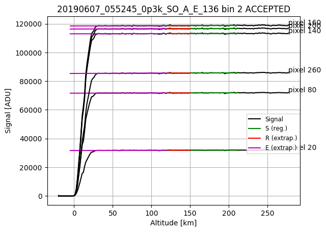
Figure 20: Each solar occultation spectrum is split into 5 regions, S, R, E, U (umbra – no signal) and T (atmosphere), corresponding to a given tangent altitude range.

 

 

2.2.21.2   YFit, YErrorFit, YErrorFitNorm – Linear regression, smoothed pixel-by-pixel gradient

The advantage of the Trompet et al. 2016 method is that the linear regression accounts for the change in brightness of the sun during the occultation, which occurs when the part of the sun being measured changes due to spacecraft pointing inaccuracies and rotation of the boresight around the centre of the sun. The transmittance is always very close to 1 at the top of the atmosphere using such a regression.

The disadvantage, however, is that the regressions are calculated pixel-by-pixel, and so the presence of shifting solar lines (due to heating of the diffraction grating, the spectral calibration of the pixels can change) complicates the fit. Such shifts should be accounted for in the retrieval algorithm, where they can be successfully modelled, and hence their presence should not be altered by the transmittance calculation. To achieve this, the gradient of each regression is itself fit using a polynomial, so that outliers due to solar line shifts are not modified. This retains the solar line effects, to be modelled out later, and also retains the regression so that boresight  pointing/rotation effects don’t affect the transmittance. Transmittance YFit is found in the same way, by dividing the spectra in the atmospheric region by the extrapolation region E.

YErrorFit and YErrorFitNorm follow the same calculation method as for YError and YErrorNorm, but using YFit spectra in the U and S regions.

 

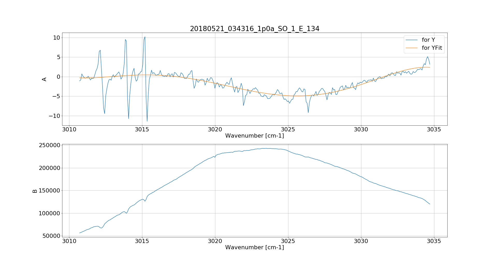
Figure 21: Polynomial fit to the linear regression gradients (A term in y = Ax + B) showing how the solar line features remain whilst the general shape is removed.

 

 

2.2.21.3   YMean, YErrorMean, YErrorMeanNorm – No linear regression

The third type is a simple mean, where each spectrum in the T region is divided by a mean of those at the top of the atmosphere to make YMean. This means that which fully retains the solar line shifts but has no linear regression, hence the transmittance may not be equal to 1 at the top of the atmosphere. YErrorMean and YErrorMeanNorm follow the same calculation method as for YError and YErrorNorm, but using YMean spectra in the U and S regions.

 

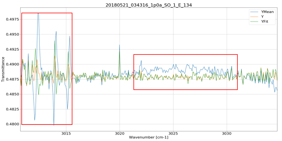
Figure 22: Transmittances calculated using the three methods. The spikes on the left are due to solar lines shifting from one pixel to another as the field of view moves from viewing the top of atmosphere to the atmosphere.

 

 

2.2.22   Level 1.0A - LNO nadir/limb radiance calibration

LNO radiometric calibration is performed using a look-up table derived from laboratory measurements made during the ground calibration campaign, potentially combined with in-flight solar measurements in future. The look-up table contains radiance-to-counts conversion values for all pixels in all diffraction orders (Figure 18).

The sensitivity of the instrument varies by diffraction order – higher orders (165 – 190) have a higher sensitivity, whereas around order 150 it has a minimum sensitivity as shown in Figure 19. This affects the choice of diffraction orders used in flight, particularly for LNO where the signal is low. Radiance values are stored in the Y dataset with the units of W/cm^-2/sr/cm^-1.

At present the error is calibrated directly from the data, using the first 50 pixels of the first uncalibrated spectrum (in counts) of the observation. A polynomial is plotted through the selected data, and this is subtracted from the data to remove the continuum shape. A standard deviation is then calculated as a single value (in counts) for the whole observation, and converted to radiance for every pixel using the look-up table. Values are stored in YError. An SNR is calculated for every pixel of every spectrum by dividing Y by YError.

Description to be modified when LNO radiometric calibration is improved.

 

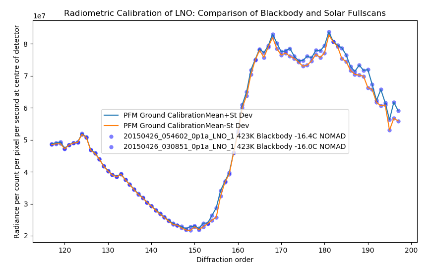
Figure 23: Radiance to counts conversion for different diffraction orders, measured at the centre of the detector. This corresponds to the sensitivity curve of the LNO channel. The lines correspond to the minimum and maximum values measured during multiple blackbody measurements.

 

 

2.2.23   Level 1.0A - UVIS nadir radiance calibration

Convert detector pixel counts into radiance (W/m2/nm/sr) by multiplying Y by the instrumental function (determined during the ground calibration campaign) contained in a look-up table and save to Y dataset. Set YUnitFlag and YTypeFlag.
Set the errors (currently set to 100%) updating YError.