LNO Dayside Nadir
The LNO dataset has been reprocessed to add a reflectance factor calibration to all files and to improve the spectral calibration. The LNO dayside nadir files now have two observation types, "DP" and "DF", which stand for "dayside nadir pass" and "dayside nadir fail". For example:
- 20180421_005020_1p0a_LNO_1_DP_169.h5
- 20180421_005020_1p0a_LNO_1_DF_164.h5
"Pass" indicates that both the diffraction order contains solar lines (to fit the solar reference spectra) and the nadir data contains solar and/or atmospheric absorption lines of sufficient depth that the pipeline was able to detect them and correctly shift both the solar and nadir spectral calibrations to match the lines. These files contain the best calibration.
"Fail" indicates that either:
- the diffraction order does not contain sufficiently deep solar lines to detect and correct the solar reference calibration
- the nadir data in the file does not contain any solar and/or atmospheric absorption lines of sufficient depth to detect and correct the solar reference calibration
- the nadir data in the file is too noisy to fit any solar or molecular lines.
In these cases, the spectral calibration has been estimated from the temperature of the LNO channel rather than a fit to absorption lines.
A fail does not necessarily mean that the data is not correct, however more care should be taken when interpreting the data - the spectral calibration is likely to be less accurate and there may be residuals in the data where solar lines have not be correctly divided out during the reflectance factor calculation.
LNO nadir HDF5 datasets
Below is a description of the new or important datasets in the LNO nadir files:
| Dataset | Description |
| Science/YReflectanceFactorOld |
The old version of the reflectance factor calibration. The baseline here is curved. |
| Science/YReflectanceFactor |
The new version of the reflectance factor calibration using all solar calibration observations (as of January 2023), with all diffraction orders converted and improved calibration at the edges of the detector. The spectra are calibrated in reflectance factor, where reflectance factor = pi * normalised nadir counts / normalised solar counts / solar-to-nadir scaling factor / cosine(Geometry/MeanIncidenceAngle). The baseline here is curved. |
| Science/YReflectanceFactorFlat | Flattened reflectance factor (using the new calibration), where a temperature dependent curve has been fitted to all spectra to reduce the curvature in the spectra. The curve is removed systematically from all spectra, so rare spectral features are retained in the data. |
| Science/YReflectanceFactorBaseline Removed | Flattened reflectance factor, using the method of Guillaume (fit to solar irradiance spectrum and individual baseline correction of each spectrum). Note that wide spectral features may be removed by this flattening technique. |
| --- | --- |
| Science/YRadiance |
The "Y" dataset from previous files. This is the radiance calculated from laboratory blackbody measurements, which uses the AOTF and blaze functions to calculate the full radiance hitting each pixel to derive the counts-to-radiance conversion. This should be used with caution, because 1) it relies on having correct AOTF and blaze functions; and 2) because the blackbody data used for the calibration is not reliable at high diffraction orders (as the planck function decreases and so the signal becomes very small). |
| Science/YRadianceSimple |
The "YAtWavenumber" dataset from previous files. This is the radiance calibrated from laboratory blackbody measurements without using the AOTF or blaze functions. The counts to radiance conversion is derived from a simple planck function at the temperature of the blackbody and wavenumber of the pixel. This calibration can also be unreliable for high diffraction orders. |
| Science/YRadianceError | Error in the YRadiance dataset, taken from a fit to the continuum in the first 50 pixels |
| Science/SNRRadiance | Radiance SNR, i.e. YRadiance/YRadianceError |
| Science/YUnmodified | Raw counts unmodified from the level 0.3A HDF5 file |
| Science/YNormalisedCounts | Raw nadir counts, normalised to counts per pixel per second |
| --- | --- |
| Geometry/MeanIncidenceAngle | Mean incidence angle (1 value per spectra). It is the mean of the Point0 - Point5 IncidenceAngle values for that spectrum. |
| --- | --- |
| Criteria/LineFit/NumberOfLinesFit | Number of molecular/solar lines in the nadir data that were successfully fit |
| Criteria/LineFit/ChiSqError | A number indicating the quality of the solar/molecular line fit (higher means the fit was better) |
| Criteria/LineFit/Error | 0=fit failed, 1=fit passed |
| --- | --- |
| Channel/MeasurementTemperature | Mean LNO baseplate temperature during the observation, taken from the TGO temperature readouts |
| --- | --- |
| Temperature/TemperatureDateTime | Datetimes for the temperature measurements in this dataset group. Temperatures start 10 minutes before the observation begins and end ten minutes after |
| Temperature/NominalSO | Temperature of the SO channel as recorded by TGO. The value is set to -999.0 if no data was recorded |
| Temperature/NominalLNO | Temperature of the LNO channel as recorded by TGO. The value is set to -999.0 if no data was recorded |
| Temperature/NominalUVIS | Temperature of the UVIS channel as recorded by TGO. The value is set to -999.0 if no data was recorded |
| Temperature/RedundantSO | Temperature of the SO channel (redundant sensor) as recorded by TGO. The value is set to -999.0 if no data was recorded |
| Temperature/RedundantLNO | Temperature of the LNO channel (redundant sensor) as recorded by TGO. The value is set to -999.0 if no data was recorded |
UVIS Occultation
UVIS grazing occultations have recently been added to the ftp in the hdf5_level_1p0a directory. Each grazing occultation is split into two separate files, one for the ingress (from the top of atmosphere up to the minimum tangent altitude) and one for the egress (up to the top of atmosphere). Hence two filenames, GI and GE respectively are required, for example:
- 20180508_024553_1p0a_UVIS_GI
- 20180508_024553_1p0a_UVIS_GE
HDF5 datasets
Several different algorithms are used to convert the UVIS occultation data to transmittance. The table below lists the dataset names and a description of each.
| Science/Y |
Transmittance is computed using a linear extrapolation of the "Sun region" (i.e. where the tangent point is above the atmosphere) for each pixel individually. This method attempts to correct for limb darkening: during a solar occultation, the pointing is not fixed on the same region of the solar disk, and so the signal from the Sun can increase or decrease as the field of view moves towards the centre or edge of the solar disk. This results in a sloped Sun region which is then fit with a linear line of best fit and extrapolated into the "Penumbral region" (i.e. where the tangent point is passing through the atmosphere). The extrapolation is then used to calculate a solar reference spectrum to calibrate each spectrum measured when the line of sight passes through the atmosphere. See Trompet et al. for a more detailed description. Advantages: the limb darkening effect is reduced by the linear extrapolation Disadvantages: the extrapolation is done separately for each pixel, therefore noisy pixels could be fit badly, resulting in a poor extrapolation. |
| Science/YMean |
The solar reference spectrum is computed per pixel by taking the mean of all the spectra in the defined "Sun region" (i.e. where the tangent point is above the atmosphere). Advantages: this method averages together multiple spectra, and so the solar reference spectrum is less noisy and less prone to extrapolation errors due to noisy pixels. Disadvantages: if the "Sun region" is not flat, e.g. due to limb darkening, the solar reference spectrum used to convert all the atmospheric spectra to transmittance will be too high or low. The transmittance should be 1.00 above the atmosphere, but if limb darkening is not accounted for, the calculated transmittances will be higher or lower than this value. => this is the agreed dataset used by the team |
| Science/YFit <unused> | Transmittance computed using a linear regression of the Sun region for each pixel individually. The gradient coefficients (A in Ax+B) are fitted using a 6th order polynomial. This method attempts to reconcile the two methods above: the extrapolation is performed per pixel, but the gradient calculated for each pixel is effective smoothed so that a pixel cannot have a very different gradient to its neighbouring pixels. This aims to correct badly fit extrapolations e.g. those on noisy pixels. |
| Science/YError | Uncertainties on Y |
| Science/YErrorMean | Uncertainties on YMean |
| Science/YErrorFit <unused> | Uncertainties on YFit |
| Science/YErrrorNorm <unused> | Uncertainties on Y, except that the solar reference spectra are normalised before the standard deviation is made. This dataset is present to remove a known issue in the SO channel calibration. |
| Science/YErrorMeanRMS | M. Wolff error analysis, version 2 (with 2nd derivative constraint) |
|
Science/YErrorMeanRandom |
Random errors as propagated through the various stages of the data pipeline => this is the agreed dataset used by the team |
| Science/YErrorMeanSystematic | Systematic errors (i.e. straylight) as propagated through the various stages of the data pipeline |
| Science/YUnmodified | Pixel counts before conversion to transmittance |
SO Occultation
HDF5 datasets
Several different algorithms are used to convert the SO occultation data to transmittance. The table below lists the dataset names and a description of each.
| Science/Y |
Transmittance is computed using a linear extrapolation of the "Sun region" (i.e. where the tangent point is above the atmosphere) for each pixel individually. This method attempts to correct for limb darkening: during a solar occultation, the pointing is not fixed on the same region of the solar disk, and so the signal from the Sun can increase or decrease as the field of view moves towards the centre or edge of the solar disk. This results in a sloped Sun region which is then fit with a linear line of best fit and extrapolated into the "Penumbral region" (i.e. where the tangent point is passing through the atmosphere). The extrapolation is then used to calculate a solar reference spectrum to calibrate each spectrum measured when the line of sight passes through the atmosphere. See Trompet et al. for a more detailed description. Advantages: the limb darkening effect is reduced by the linear extrapolation Disadvantages: the extrapolation is done separately for each pixel, therefore noisy pixels could be fit badly, resulting in a poor extrapolation. => this is the agreed dataset used by the team |
| Science/YMean |
The solar reference spectrum is computed per pixel by taking the mean of all the spectra in the defined "Sun region" (i.e. where the tangent point is above the atmosphere). Advantages: this method averages together multiple spectra, and so the solar reference spectrum is less noisy and less prone to extrapolation errors due to noisy pixels. Disadvantages: if the "Sun region" is not flat, e.g. due to limb darkening, the solar reference spectrum used to convert all the atmospheric spectra to transmittance will be too high or low. The transmittance should be 1.00 above the atmosphere, but if limb darkening is not accounted for, the calculated transmittances will be higher or lower than this value. |
| Science/YFit | Transmittance computed using a linear regression of the Sun region for each pixel individually. The gradient coefficients (A in Ax+B) are fitted using a 6th order polynomial. This method attempts to reconcile the two methods above: the extrapolation is performed per pixel, but the gradient calculated for each pixel is effective smoothed so that a pixel cannot have a very different gradient to its neighbouring pixels. This aims to correct badly fit extrapolations e.g. those on noisy pixels. |
| Science/YError |
Uncertainties on Y, except that the solar reference spectra are normalised before the standard deviation is made. => this is the agreed dataset used by the team |
| Science/YErrorMean |
Uncertainties on YMean |
| Science/YErrorFit | Uncertainties on YFit |
| Science/YErrorCovariance | Uncertainties calculated using a covariance matrix to remove systematic errors, leaving only the random error. As presented by Adrian and Miguel at SWT#22 |
| Science/CovarianceMatrix | The covariance matrix used to calculate the dataset Science/YErrorCovariance |
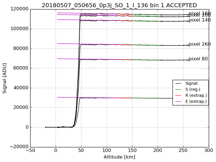
Science/Y example for an SO channel observation
Note that the Sun region is not flat, therefore the extrapolated line has a small negative gradient
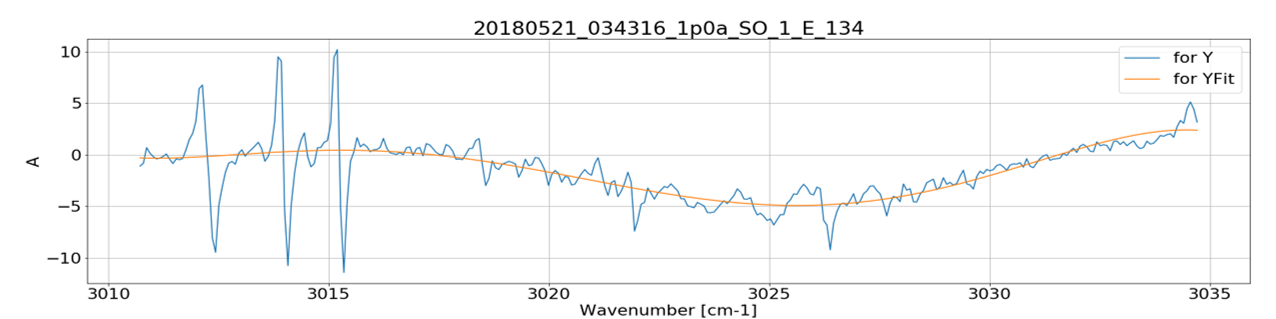
Science/YFit example for an SO observation
Here the gradient calculated for every pixel (blue) is fit by a polynomial (orange) so that any gradients much larger or smaller than their neighbouring pixels are smoothed. Here the large changes in gradient are caused by solar lines that are shifting slightly due to small changes in the instrument temperature (the spectral calibration is dependent on instrument temperature for SO and LNO). For UVIS this effect should be negigible - however bad gradients due to noisy pixels will be smoothed also.
SO spectral calibration: updated coefficients in the HDF5 files
| Channel/AOTFCentralWavenb | AOTF centre in cm-1 from Villanueva et al. 2022 |
| Channel/AOTFFunction |
4 parameters from Villanueva et al. 2022:
|
| Channel/AOTFOrderCoefficients | Coefficients to calculate order from AOTF frequency (unchanged from previous version) |
| Channel/AOTFWnCoefficients | Recalculated in data pipeline from new AOTF central wavenumbers |
| Channel/SpectralResolution |
5 parameters from Villanueva et al. 2022:
|
| Channel/BlazeFunction |
6 coefficients:
|
| Science/X | Wavenumber of each pixel from Trompet et al. 2022 |
| Channel/PixelSpectralCoefficients | Pixel and order to wavenumber coefficients from Trompet et al. 2022 |
| Channel/FirstPixel | Calculated pixel shift due to temperature from Trompet et al. 2022 |
SO/LNO/UVIS Solar Calibrations
HDF5 files now pass through the pipeline to level 1.0a
HDF5 filenames
Calibration files are assigned additional letter, so miniscans / fullscans / linescans / solar pointings etc. can be distinguished directly from the filename
CM = miniscan
CF = fullscan
CL = linescan
Spectral calibration added to solar fullscans / linescans / pointings (not miniscans)
Y data converted to 2D array to match all other observation files