JGR (2022); https://doi.org/10.1029/2022JE007346

M. A. J. Brown, M. R. Patel, S. R. Lewis, J. A. Holmes, G. J. Sellers, P. M. Streeter, A. Bennaceur, G. Liuzzi, G. L. Villanueva, A. C. Vandaele

We show a positive vertical correlation between ozone and water ice using a vertical cross-correlation analysis with observations from the ExoMars Trace Gas Orbiter's Nadir and Occultation for Mars Discovery instrument. This is particularly apparent during LS = 0°–180°, Mars Year 35 at high southern latitudes, when the water vapor abundance is low. Ozone and water vapor are anti-correlated on Mars; Clancy et al. (2016, https://doi.org/10.1016/j.icarus.2015.11.016) also discuss the anti-correlation between ozone and water ice. However, our simulations with gas-phase-only chemistry using a 1-D model show that ozone concentration is not influenced by water ice. Heterogeneous chemistry has been proposed as a mechanism to explain the underprediction of ozone in global climate models (GCMs) through the removal of HOx. We find improving the heterogeneous chemical scheme by creating a separate tracer for the HOx adsorbed state, causes ozone abundance to increase when water ice is present (30–50 km), better matching observed trends. When water vapor abundance is high, there is no consistent vertical correlation between observed ozone and water ice and, in simulated scenarios, the heterogeneous chemistry has a minor influence on ozone. HOx, which are by-products of water vapor, dominate ozone abundance, masking the effects of heterogeneous chemistry on ozone, and making adsorption of HOx have a negligible impact on ozone. This is consistent with gas-phase-only modeled ozone, showing good agreement with observations when water vapor is abundant. Overall, the inclusion of heterogeneous chemistry improves the ozone vertical structure in regions of low water vapor abundance, which may partially explain GCM ozone deficits.

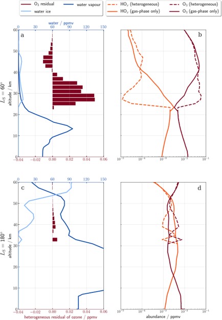
Modeled profiles from the 1‐dimensional Martian Photochemical Modelof (a and b) low water vapor (at LS = 60°), and (c and d) high water vapor (at LS = 180°) at latitude 0°, local solar time 1200 hr (First column; a and c) vertical profiles of (light blue) water ice, (dark blue) water vapor, and (dark red bars) the ozone residual (calculated by subtracting the heterogeneous ozone from the gas‐phase only ozone). Abundance difference for ozone is on the bottom x‐axis and abundance for water ice and vapor is on the top x‐axis. (Second column; b and d) vertical profiles of (dark red) ozone and (orange) HOx for (dashed) heterogeneous and (solid) gas‐phase‐only simulations. Note the abundances are on a logarithmic scale.